Clustering with Mean Shift

Introduction

I came across this handy and intricate unsupervised learning algorithm few months ago on a work (to appear) where we want to do something similar on some non-linear manifolds. Contrary to the ubiquitous Lloyd (a.k.a. $k$-means) algorithm, mean shift does not require any prior knowledge or tuning of cluster numbers. I later wrote a simple few liner in C++ to experiment it with planar toy data. Code for this blog is available at GitHub.

Mean shift is categories as one of the unsupervised kernel density estimation methods for clustering. Speaking of density estimation, mainly we consider two general categories, parametric and non-parametric. Notable examples of the former include the familiar MLE, MAP, or BMA, where models are parametrized explicitly. The latter encompasses $k$-NN, kernel density estimation and so forth. As an interesting side-note, often we consider neural networks of a fixed architecture as parametric models. Some works have been done to reduce the hyperparameters and make it more non-parametric, for examples, in a recent ICLR [Philipp and Carbonell 2017].

The Algorithm

Density Estimation

Given a set of datapoints ${\boldsymbol{x}}_{i=1}^N$, where $\boldsymbol{x} \in \mathcal{R}^k$, we are interested in investigating the underlying data generating distribution $f(\boldsymbol{x})$, which is, unfortunately, unknown. If we may obtain some (good estimation) of the density, we can then find its modes and cluster the observations in accordance with the proximity to the modes.

This intuition suggested a two-step iterative algorithm for such maneuver. Concretely, assume the underlying data lying on some metric space with metric $d$ (hence the notion of proximity is well defined via, e.g., $\mathcal{l}_2$ norm in $\mathcal{R}^k$), which is differentiable; With proper kernel function $K(\cdot)$ chosen as a smoother, the kernel density estimator is given as [Fukunaga and Hostetler 1975]:

$$\hat{f}(\boldsymbol{x}) = \frac{c}{Nh^k} \sum_{i=1}^N K \left( \frac{ d(\boldsymbol{x}, \boldsymbol{x}_i)}{h}\right ),$$

where $h$ the bandwidth (since it determines the window of the kernel smoother, as we shall see later), $c$ is the normalizing constant.

Choices of Kernel Function

In the original paper of Fukunaga and Hostetler, several regularity conditions must apply for some function to be a valid kernel function including integrated to unity ($\int K(\boldsymbol{x})) \mathrm{d} \boldsymbol{x} = 1$), no singularities ($ \sup\lvert K(\cdot) \rvert \lt \infty$), $\int \lvert K(\boldsymbol{x}) \rvert \lt \infty$ and $\lim_{\lVert \boldsymbol{x} \rVert \to \infty} \lVert\boldsymbol{x}\rVert^k K(\boldsymbol{x}) = 0$.

Note we define the kernels as a function from $\mathcal{R}$ to $\mathcal{R}$. That is, we take norm before feeding data to the kernel. In practice, we generally use three kernels, namely:

• Gaussian Kernel

Most often, we require the covariance matrix being identity, hence:

$$K(x) = \frac{1}{\sqrt{2\pi}} \exp\{-\frac{1}{2}\lVert x\rVert ^ 2\}.$$

• Uniform Kernel

$$K(x) = 1\{\lVert x\rVert \lt 1 \}.$$

• Epanechnikov Kernel

$$K(\boldsymbol{x})= \frac{3}{4}(1-\lvert x \rvert ^2) 1\{\lvert x \rvert \lt 1 \}.$$

Noted in the case of uniform and Epanechnikov kernels, we limit their supports to be $[0,1]$, hence the hyperparameter $h$ hinted earlier is indeed controlling the window of the smoother.

Mode Seeking via Gradient

Recall to find the mode, we equate the gradient of the density to zero. Define $g(x) = -\frac{\partial}{\partial \boldsymbol{x}} K(x)$, we have that:

$$\begin{aligned} \hat{\nabla f(\boldsymbol{x})} &= - \frac{1}{Nh^k} \sum_{i=1}^N \nabla d^2(\boldsymbol{x}, \boldsymbol{x_i}) g \left( \frac{d^2( \boldsymbol{x}, \boldsymbol{x_i})}{h^2} \right) \\ &= -\frac{1}{Nh^k} \sum_{i=1}^N \left\{ \frac{\sum_{i=1}^N g \left( \frac{d^2(\boldsymbol{x}, \boldsymbol{x_i})}{h^2}\right) \nabla d^2(\boldsymbol{x}, \boldsymbol{x_i})} {\sum_{i=1}^N g \left( \frac{d^2(\boldsymbol{x}, \boldsymbol{x_i})}{h^2}\right)} \right\}. \end{aligned}$$

This is indeed a very general result, and has some subtle implications: to perform mean shift, it suffices to have metrics that is square-differentiable. This generalizes to piecewise differentiable metrics.

For example, using canonical Euclidean norm, we have that:

$$\begin{aligned} \hat{\nabla f(\boldsymbol{x})} &= \frac{2c}{Nh^k} \sum_{i=1}^N g \left( \frac{\lVert \boldsymbol{x} - \boldsymbol{x}_i \rVert ^ 2}{h^2} \right) \left\{ \frac{\sum_{i=1}^N \boldsymbol{x}_i g \left( \frac{\lVert \boldsymbol{x} - \boldsymbol{x}_i \rVert ^2}{h^2}\right) } {\sum_{i=1}^N g \left( \frac{\lVert \boldsymbol{x} - \boldsymbol{x}_i \rVert ^ 2}{h^2}\right)} - \boldsymbol{x} \right\}. \end{aligned}$$

What does this suggest? Given a point, the first term is constant, hence only the second term matters in our iterative procedure. Define

$$\boldsymbol{m} = \left\{ \frac{\sum_{i=1}^N \boldsymbol{x}_i g \left( \frac{\lVert \boldsymbol{x} - \boldsymbol{x}_i \rVert ^ 2}{h^2}\right) } {\sum_{i=1}^N g \left( \frac{\lVert \boldsymbol{x} - \boldsymbol{x}_i \rVert ^ 2}{h^2}\right)} - \boldsymbol{x} \right\},$$

the mean shift vector, which can be perceived as a smoothed centroid of ${\boldsymbol{x}}$; setting $\hat{\nabla f} (\boldsymbol{x}) = 0$ thus amounts to seek the centroids under the kernel smoother $g(\cdot)$. Since $g(\cdot)$ is the actual kernel we use to weigh the points, it is commonly called the “shadow” of the original kernel $K(\cdot)$.

Relationship between EM

If we further consider the “real” centroids as missing data, the above optimization problem can be cast as a variant of EM algorithm. Concretely, in E-step, we take expectations conditioning on the previously sought centroids of the smoother. That is, in fact:

$$\sum_{i=1}^N f (\boldsymbol{x}_i) = \boldsymbol{E} \left[ F \vert \left\{\boldsymbol{x}_c\right\}\right],$$

where ${ \boldsymbol{x}_c }$ are observed centroids (from last iterations), and $F$ is the actual objective in terms of the real unknown centroids expressed as a KDE. Hence in the subsequent M-step, the only work to be done is to equal the gradient to zero to complete one EM iteration.

The major difference is whether the estimated results are fed to the next iteration. To be precise, there are typically two types of mean shifts: one in which the modes are not to replace the data points, which is commonly used for clustering; the other one being substituting the data points for the learnt modes, which can be used for image segmentation.

In the latter case, the mean shift can be readily regarded as within the EM paradigm.

Concrete Examples

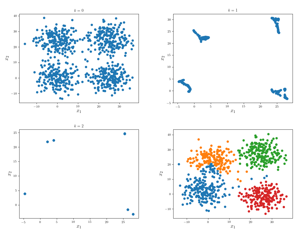
We consider a simple examples: four mixed Gaussian that is visually well separable:

We first run one iteration using Gaussian kernel with bandwidth 18 and pruning criterion 18. These hyperparameters are highly problem dependent.

We can see the modes of four clusters shrink largely together. Hence applying a pruning algorithm such as DFS would do the trick:

In practice, one may alter the learning parameters and perform several iterations of the whole algorithm. Nonetheless, since the problem is ill-posed per se, it would be better to visualize the results to determine which result is most desirable.

For example, consider the following ring data (data source):

The following results are generated from different sets of configurations:

References

1. Fukunaga, K. and Hostetler, L. 1975. The estimation of the gradient of a density function, with applications in pattern recognition. IEEE Transactions on information theory 21, 1, 32–40.
2. Philipp, G. and Carbonell, J.G. 2017. Nonparametric Neural Networks. ICLR ’17.