Transfer Learning via Geodesic Sampling
Introduction
In our recent magazine paper (under review), one topic of interests is subspace-aided transfer learning. In this blog, we give an overview of the method we studied with illustrations that are not included in the paper. This blog will nonethless not go into mathematics details, rather, we ask motivated readers to bear with the partial presentation and postpone the enjoyment of full derivation when our paper is ready. We hope our vivid illustrations and animations may partially explain the reasons why this seemingly ad-hoc method may work a posteriori.
More introductory texts on transfer learning can be found in one of my earlier blog. We should remark that, the jargon “domain adaptation” and “transfer learning” are not exactly equivalent in a mathematical sense. Subtle differences exist though, which are essentially different assumptions on the underlying latent distribution. We do not, nonetheless, differentiate them in this rather casual writing.
Dataset
As a general setup, there are several popular dataset tailored for benchmarking transfer learning. We select the celebrated Office data set [Saenko et al. 2010] augmented by Caltech-256 [Griffin et al. 2007]. These datasets have been collected for many years and are among the very popular choices.
Office dataset contains a handful of categories of objects whose images are collected by either from online merchant (‘amazon’); by a DSLR camera (‘dslr’); or by a webcam (‘webcam’). The Caltech-256 dataset, as the name suggested, contains 256 categories of objects. Usually, we would select a small subset of categories in common, and train a supervised model using one domain out of the four and test in another domain. This procedure is known as unsupervised domain adaptation since no label in the target domain is known; Alternatively, if we train the model using very few but not none data from the target domain in addition to the source domain, we are indeed doing the semi-supervised (or semi-unsupervised) domain adaptation.
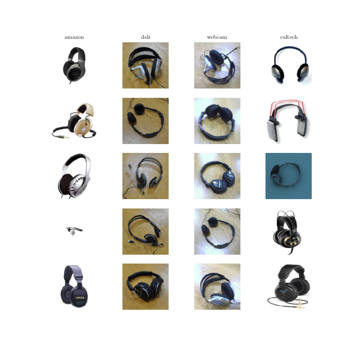
Firstly, let us have a brief overview of several categories among four domains:
Headphone
Projector
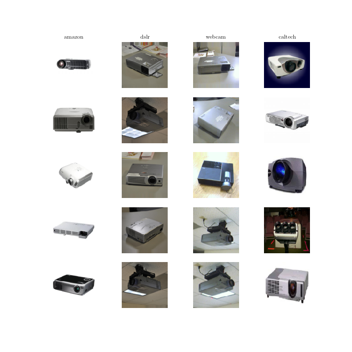
As suggested by name, we see the core disparities between domains: “amazon” has generally better-aligned objects; images in “dslr” are of higher resolution; “webcam” on the contrary is much more casual and usually under unbalanced illumination; “caltech” is more in the wild. The discrepancies here can be considered as a new scenario that we wish our model to generalized well from previously learnt domains.
Geodesic Sampling
The details of the methods we studied and implemented can be found in [Gopalan et al. 2011; Gong et al. 2012]. Very roughly speaking, we model the source and target domains of images of the same category as two points on some highly-nonlinear manifold (i.e., Grassmann manifold), which, by some heurstic argument, may capture the geometric and statistical properties of the set of the image by rendering a unified latent representation. Though the manifold is highly non-linear per se, its distinct element infact constitutes of vector spaces (i.e., linear subspaces); we may as well construct its tangent space as vector spaces. Furthermore, to measure the discrepancies between points (or rather, define the metric over the manifold), we progress to the notion of principle angles between subspaces. For example, in $\mathcal{R}^2$, each vector is by itself (the basis of) a 1 dimensional subspace and thus the discrepancy between two such spaces can be measured by the cosine of the angle they make. Principle angle is a natural extension of such construction in general dimension subspaces. Above is some very coarse-grained discussion, we refer interested readers for classical texts on the subjects such as Boothby, Edelman or Absil. Readers are also encouraged to check out our paper for abundant details omitted here.
The geodesic is the shortest curve under constant velocity joining two points (the velocity is indeed the element of the tangent space). By sampling on the geodesic between the source and target domains, it has been heuristically argued and empirically tested that some intermediate points exhibited more consistency in terms of statistical and geometrical properties between source and target domains. Such samples can thus be viewed as latent representations and consequently a discriminatively-trained classifier should be able to generalize well on such latent spaces.
In fact, suppose we parametric the geodesic (recall it is simply a curve joining two points) in terms of $t \in [0, 1]$, we can infact visualize the change of a single image in the source domain as we traverse the geodesic to another domain. For such maneuver, we apply a similar procedure used in “Eigenfaces” by way of principle component analysis.
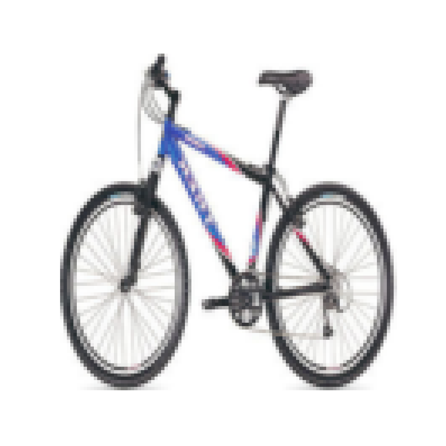
Concretely, assume we wish to generalize bikes from “caltech” to “amazon”, we first plot their mean images to have a better feeling of the two domains:
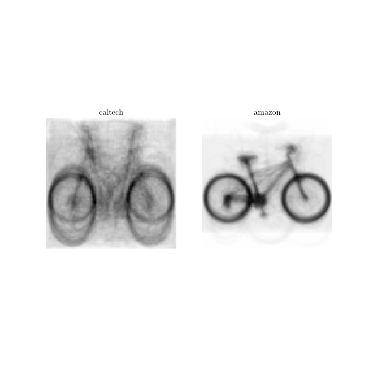
The mean image is simply an average over all images in the domain, we noted the main differences may be the size of the wheels and orientation of the bikes; and the characteristics shared are the structures of the bike.
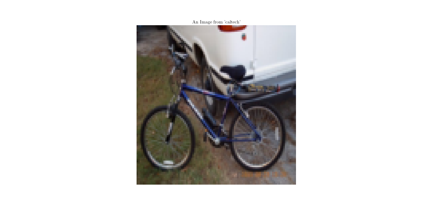
We choose an image from the source domain and visualize its latent-representation on five samples along the geodesic:
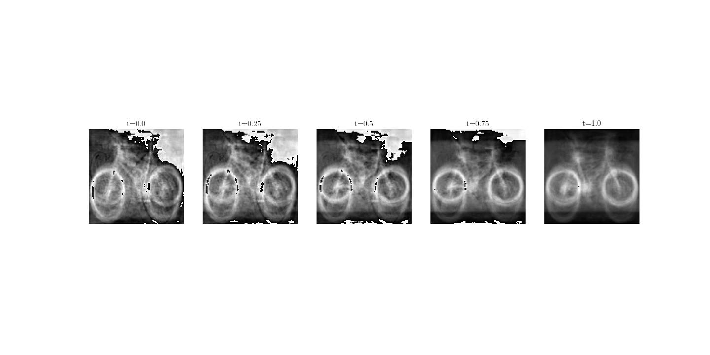
The result shows some interesting features besides the overreacted pixels: along the geodesic, there is a noticeable deformation of the front wheel shrinking to the size that mostly appears in the target domain.
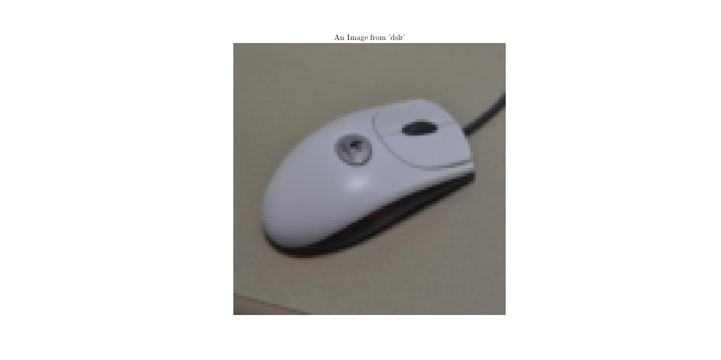
As another example, consider the computer mouse from “dslr” to “webcam”:
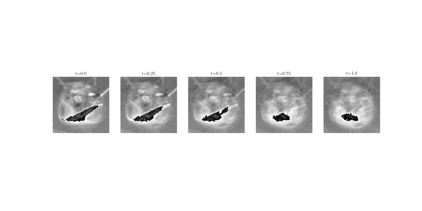
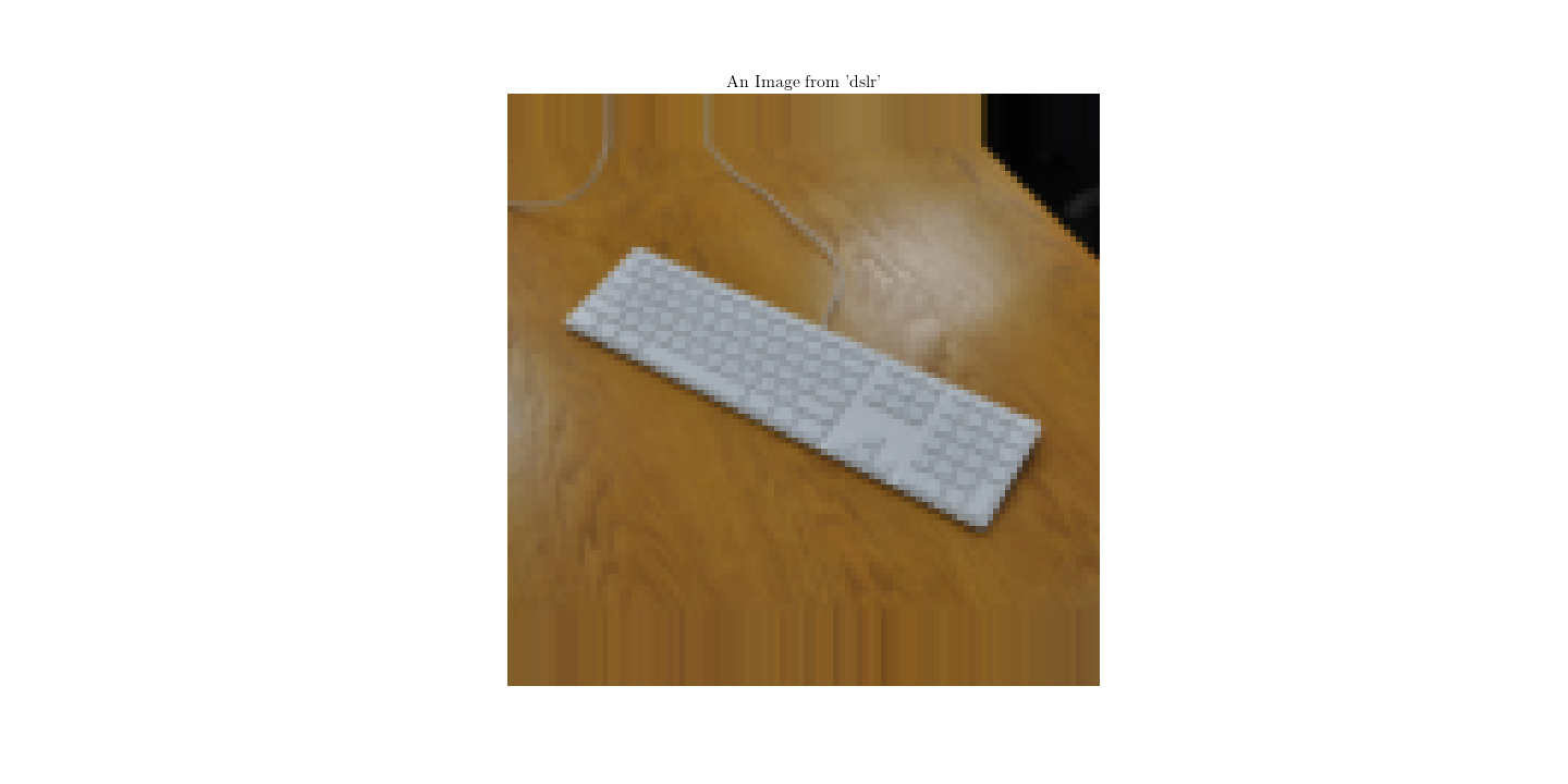
and keyboards of the same source-target pair:
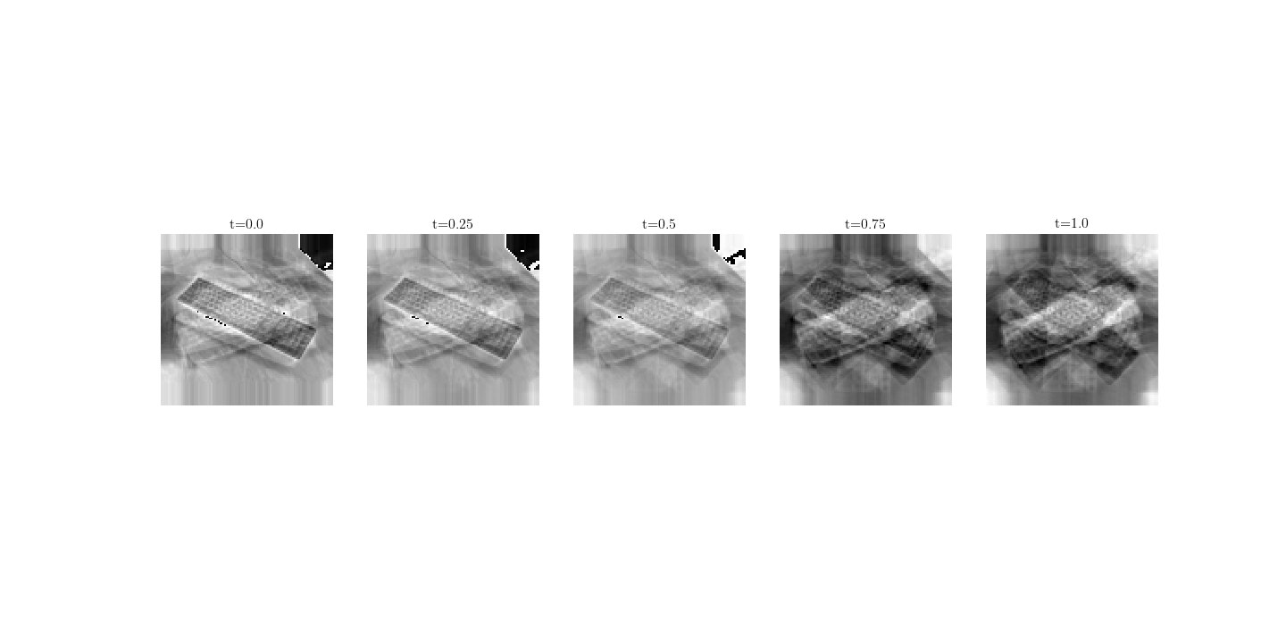
This example illustrates that one of the defining factors of the visual consistency of such manuvour is the quality of the mean image.
In fact, we can animate the whole process, take our now familiar caltech bike, for example:
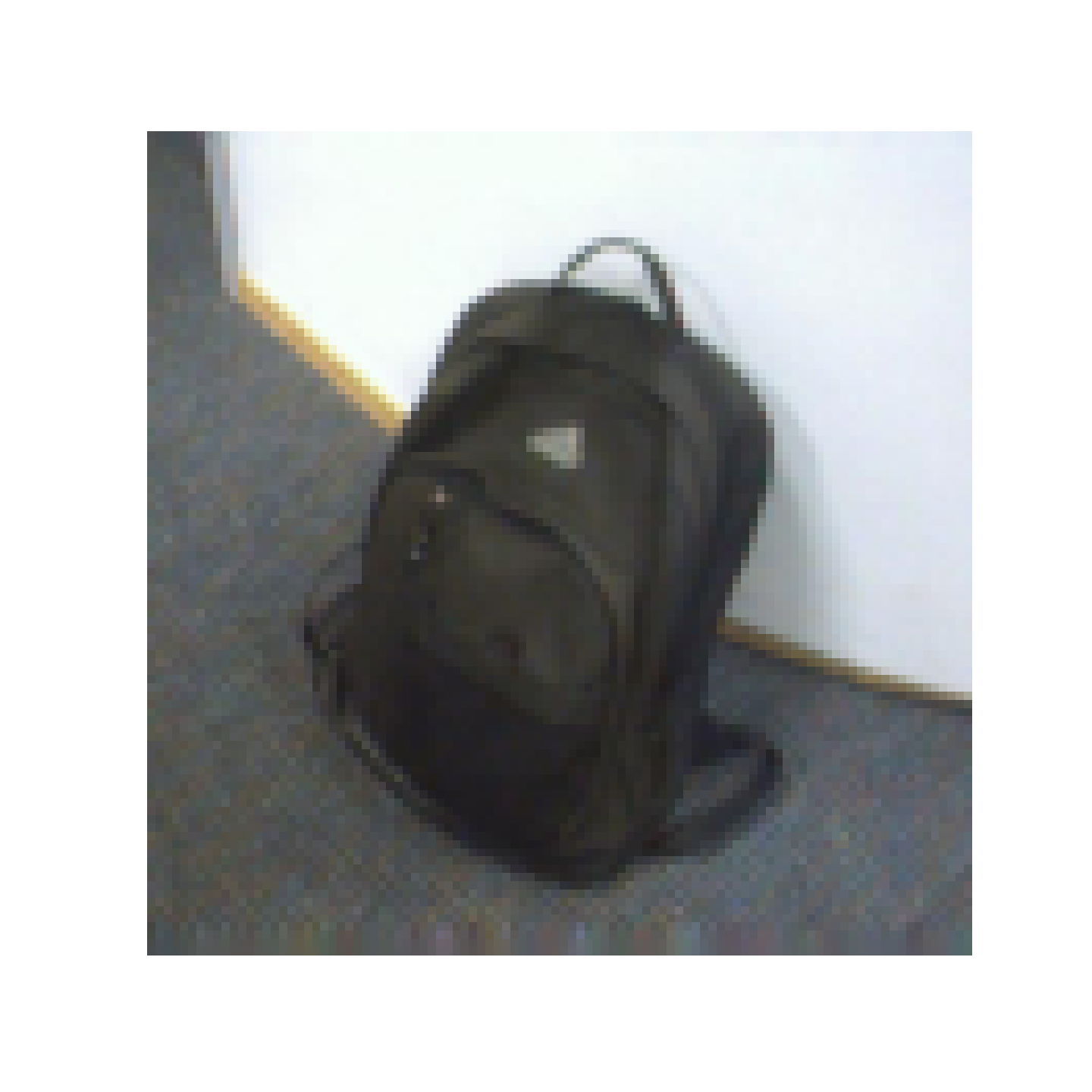
How about a backpack from “webcam” to “amazon”?
Feature Visualization
Going along this direction a little bit further, we are curious what are the latent features and how they change along the geodesic. To do this, we follow the same procedure of “Eigenface” again. Concretely, we animate top eigenvector of the latent samples along the geodesic of calculators from “dslr” to “amazon”.
Remark.
During a recent talk by D. A. Forsyth I attended, he commented on a general perception in CV community which I consider to be very true:
In the past, we understood the theories very well, but we cannot do well; now the models perform very well but we do not know why.
I believe the incorporation of deep models and mechanism inspired from geometrically/physcially-based perspective may lead to our better understanding and exploring the capacity of deep models; and better comprehend how to obtain models that really understand the image, not at least the classifications or regressions.
The experiments in this blog are purely illustrative: we did not even bother to feed HOG or SURF features, rather, we directly used normalized raw images; we did neither augment the dataset by removing lousy images or localizing objects.
References
- Gong, B., Shi, Y., Sha, F., and Grauman, K. 2012. Geodesic flow kernel for unsupervised domain adaptation. Computer Vision and Pattern Recognition (CVPR), 2012 IEEE Conference on, IEEE, 2066–2073.
- Gopalan, R., Li, R., and Chellappa, R. 2011. Domain adaptation for object recognition: An unsupervised approach. ICCV ’11, IEEE, 999–1006.
- Griffin, G., Holub, A., and Perona, P. 2007. Caltech-256 object category dataset. .
- Saenko, K., Kulis, B., Fritz, M., and Darrell, T. 2010. Adapting visual category models to new domains. Computer Vision–ECCV 2010, 213–226.